Deep dive into joins, pivots, string ops and more with the tidyverse
Author
David Munoz Tord
Published
May 11, 2025
Course Overview
Welcome to Tidyverse II! In this intermediate course, we’ll build upon your existing Tidyverse knowledge to tackle more complex data manipulation tasks. You’ll learn how to effectively combine, reshape, and clean diverse datasets, mastering techniques essential for real-world data analysis.
We will cover:
Recap & Setup: A quick refresher on Tidyverse fundamentals and setting up our environment.
Joins: Combining data from multiple tables.
Pivoting & Reshaping: Transforming data between wide and long formats.
String Operations: Working with textual data using {stringr}.
Date-Time Operations: Handling dates and times with {lubridate}. (Coming soon!)
Advanced Graphics: Taking {ggplot2} skills to the next level. (Coming soon!)
Factor Operations: Managing categorical data with {forcats}. (Coming soon!)
Capstone Project: Applying all learned skills to a comprehensive project. (Coming soon!)
Let’s begin!
Lesson 1: Recap & Setup
Before diving into new material, let’s briefly revisit the core principles of the Tidyverse and ensure our R environment is ready.
The Tidyverse is an opinionated collection of R packages designed for data science. All packages share an underlying design philosophy, grammar, and data structures. Key packages include:
{dplyr}: For data manipulation (filtering, arranging, selecting, mutating, summarizing).
{ggplot2}: For creating elegant and informative data visualizations.
{tidyr}: For tidying data (making it easy to work with).
{readr}: For reading rectangular data files (like CSVs).
{purrr}: For functional programming, enhancing your R toolkit.
{tibble}: For modern, user-friendly data frames.
{stringr}: For working with strings and regular expressions.
{forcats}: For handling categorical variables (factors).
A central concept is the pipe operator %>% (or the base R pipe |> from R 4.1+). It allows you to chain operations together in a readable and intuitive way, passing the result of one function as the first argument to the next.
For this course, we’ll primarily use RStudio or a similar R environment. Ensure you have the tidyverse package installed. If not, you can install it with install.packages("tidyverse").
# Load the entire tidyverselibrary(tidyverse)
── Attaching core tidyverse packages ──────────────────────── tidyverse 2.0.0 ──
✔ dplyr     1.1.4     ✔ readr     2.1.5
✔ forcats   1.0.0     ✔ stringr   1.5.1
✔ ggplot2   3.5.2     ✔ tibble    3.2.1
✔ lubridate 1.9.4     ✔ tidyr     1.3.1
✔ purrr     1.0.4
── Conflicts ────────────────────────────────────────── tidyverse_conflicts() ──
✖ dplyr::filter() masks stats::filter()
✖ dplyr::lag()    masks stats::lag()
ℹ Use the conflicted package (<http://conflicted.r-lib.org/>) to force all conflicts to become errors
# Example: Using the pipe with dplyr# Let's inspect the built-in starwars datasetstarwars_tibble <- starwars %>%as_tibble()starwars_tibble %>%glimpse()
# A quick dplyr reminder:# Find all droids taller than 100cmstarwars_tibble %>%filter(species =="Droid"& height >100) %>%select(name, height, mass, homeworld) %>%arrange(desc(height))
# A tibble: 2 × 4
  name  height  mass homeworld
  <chr>  <int> <dbl> <chr>
1 IG-88    200   140 <NA>
2 C-3PO    167    75 Tatooine
Exercise 1.1: Quick Check
Familiarize yourself again with a built-in dataset. 1. Load the tidyverse package. 2. Convert the mtcars dataset to a tibble. 3. Use glimpse() to see its structure. 4. Use head() to view the first few rows. 5. How many cars have more than 4 cylinders and achieve more than 20 miles per gallon (mpg)?
Lesson 2: Joins (Part I & II)
Often, the data you need is spread across multiple tables. Joins are how we combine these tables based on common variables (keys).
Part I: Stacking Tables
Sometimes, you don’t need to match rows based on keys, but rather stack tables on top of each other or side-by-side.
bind_rows(...): Stacks multiple data frames vertically.
It matches columns by name.
Columns that don’t exist in one of the tables will be filled with NA.
You can use the .id argument to create a new column indicating the original data frame for each row.
bind_cols(...): Stacks multiple data frames horizontally.
This is less common for typical data analysis workflows because it requires the data frames to have the same number of rows and for those rows to correspond to each other (e.g., same observations in the same order).
If column names are duplicated, bind_cols() will automatically rename them.
Notice how revenue is NA for Q1 sales, and source_table_id tells us which original table the row came from.
Exercise 2.1: Stacking Sales Data
You have three tibbles representing sales data for different regions. Combine them into a single tibble.
Part II: Relational (dplyr) Joins
These joins combine data frames based on matching values in specified “key” columns.
Key Concepts:
Primary Key: A column (or set of columns) in a table that uniquely identifies each row.
Foreign Key: A column (or set of columns) in one table that refers to the primary key in another table.
Joins work by matching foreign keys to primary keys.
Mutating Joins: Add columns from one table to another.
left_join(x, y, by = "key_column"): Keeps all rows from x and all columns from x and y. Rows in x with no match in y will have NA values in the new columns from y.
right_join(x, y, by = "key_column"): Keeps all rows from y. Rows in y with no match in x will have NA values. (Less common, often you can achieve the same by swapping x and y in a left_join).
inner_join(x, y, by = "key_column"): Keeps only rows from x that have a match in y.
full_join(x, y, by = "key_column"): Keeps all rows from both x and y. If there are no matches, NAs are inserted.
Filtering Joins: Filter rows from one table based on whether they match in another, but do not add columns.
semi_join(x, y, by = "key_column"): Keeps all rows from x that have a match in y. Does not duplicate rows in x if there are multiple matches in y.
anti_join(x, y, by = "key_column"): Keeps all rows from x that do not have a match in y. Useful for finding unmatched records.
Specifying Keys with by: * by = "key_col": If the key column has the same name in both tables. * by = c("key_col_x" = "key_col_y"): If key columns have different names. * by = c("key1", "key2"): For multiple key columns (composite key), all with same names. * by = join_by(col_x == col_y, another_x == another_y): A more flexible dplyr 1.1.0+ syntax for complex joins, including inequality or rolling joins (though we focus on equality here).
Example: left_join and inner_join
patients <-tribble(~patient_id, ~name,1, "Alice",2, "Bob",3, "Charlie")visits <-tribble(~visit_id, ~patient_id, ~visit_date,101, 1, "2023-01-15",102, 2, "2023-01-20",103, 1, "2023-02-10",104, 4, "2023-02-15"# Patient 4 not in patients table)# Left Join: Keep all patients, add visit info if availablepatients_left_visits <-left_join(patients, visits, by ="patient_id")print("Left Join (patients to visits):")
[1] "Left Join (patients to visits):"
print(patients_left_visits) # Charlie will have NAs for visit_id, visit_date
# A tibble: 4 × 4
  patient_id name    visit_id visit_date
       <dbl> <chr>      <dbl> <chr>
1          1 Alice        101 2023-01-15
2          1 Alice        103 2023-02-10
3          2 Bob          102 2023-01-20
4          3 Charlie       NA <NA>
# Inner Join: Keep only patients who had visitspatients_inner_visits <-inner_join(patients, visits, by ="patient_id")print("Inner Join (patients to visits):")
[1] "Inner Join (patients to visits):"
print(patients_inner_visits) # Charlie and Patient 4 from visits are excluded
# A tibble: 3 × 4
  patient_id name  visit_id visit_date
       <dbl> <chr>    <dbl> <chr>
1          1 Alice      101 2023-01-15
2          1 Alice      103 2023-02-10
3          2 Bob        102 2023-01-20
# Anti Join: Which patients had no visits?patients_no_visits <-anti_join(patients, visits, by ="patient_id")print("Anti Join (patients with no visits):")
[1] "Anti Join (patients with no visits):"
print(patients_no_visits) # Should show Charlie
# A tibble: 1 × 2
  patient_id name
       <dbl> <chr>
1          3 Charlie
# Semi Join: Which patients had at least one visit? (returns columns of patients only)patients_with_visits_semi <-semi_join(patients, visits, by ="patient_id")print("Semi Join (patients with visits):")
[1] "Semi Join (patients with visits):"
print(patients_with_visits_semi) # Should show Alice and Bob
# A tibble: 2 × 2
  patient_id name
       <dbl> <chr>
1          1 Alice
2          2 Bob
Exercise 2.2: Joining Orders and Customers
You have two tibbles: customers and orders. 1. Perform a left_join() to combine orders with customers data. Which orders don’t have customer information? 2. Perform an inner_join() to see only orders with valid customer information. 3. Use anti_join() to find customers who have not placed any orders.
Lesson 3: Pivoting & Reshaping Data
Data often comes in formats that are not ideal for analysis or plotting. Pivoting is the process of changing the shape of your data by turning: * Wide data into long data (pivot_longer()): This is often needed when some column names are actually values of a variable. * Long data into wide data (pivot_wider()): This is useful for creating summary tables or when variables are stored in rows.
The goal is often to achieve “tidy data” where: 1. Each variable forms a column. 2. Each observation forms a row. 3. Each type of observational unit forms a table.
pivot_longer()
Use pivot_longer() when you have data spread across multiple columns, and those column names themselves represent values of a variable.
Key arguments: * data: The data frame to reshape. * cols: The columns to pivot (gather). You can use dplyr select helpers like starts_with(), ends_with(), everything(), c(col1, col2), etc. * names_to: A string specifying the name of the new column that will store the names of the pivoted columns. * values_to: A string specifying the name of the new column that will store the values from the pivoted columns. * names_prefix: (Optional) A string prefix to remove from the column names before they become values in the names_to column. * names_sep or names_pattern: (Optional) For more complex scenarios where column names encode multiple variables. * values_drop_na = TRUE: (Optional) To drop rows where the value in the values_to column is NA.
long_data <- wide_data %>%pivot_longer(cols =starts_with("test"), # or c(test1_score, test2_score, test3_score)names_to ="test_name",values_to ="score",names_prefix ="test"# removes "test" from "test1_score" -> "1_score"# A better approach for names_prefix or names_transform might be needed for cleaner test_name )# For cleaner test names, we can use names_transform or further mutatelong_data_cleaner <- wide_data %>%pivot_longer(cols =-student_id, # pivot all columns except student_idnames_to ="test_name_raw",values_to ="score" ) %>%mutate(test_number =str_extract(test_name_raw, "\\d+")) %>%# Extract numberselect(student_id, test_number, score)print("Long Data (Simpler):")
print("Long Data (using names_pattern for more complex extraction):")
[1] "Long Data (using names_pattern for more complex extraction):"
# If columns were like test_1_score, test_2_score# wide_data_complex_names <- tribble(# ~student_id, ~test_1_score, ~test_2_score,# "S101", 85, 90,# )# long_data_pattern <- wide_data_complex_names %>%# pivot_longer(# cols = starts_with("test"),# names_to = c(".value", "test_number"), # .value takes part before _# names_pattern = "test_([0-9]+)_(.*)", # Captures number and "score"# # This is more advanced; for now, focus on simpler names_to/values_to# )# print(long_data_pattern)
Exercise 3.1: Long Format for Lab Results
You have a tibble lab_results_wide where each row is a patient, and columns represent different lab tests taken on different days (e.g., glucose_day1, hgb_day1, glucose_day7, hgb_day7). Convert this to a long format with columns: patient_id, test_type, day, value.
pivot_wider()
Use pivot_wider() when you have observations scattered across multiple rows, and you want to consolidate them into a wider format. This is the inverse of pivot_longer().
Key arguments: * data: The data frame to reshape. * names_from: The column whose values will become new column names. * values_from: The column whose values will fill the new columns. * values_fill: (Optional) A value to use if a combination of id_cols and names_from doesn’t exist (to fill explicit NAs). * id_cols: (Optional) Columns that uniquely identify each observation unit, which will be kept as is. If not specified, all columns not used in names_from or values_from are used.
You have long_summary_data with columns country, year, metric_name, value. Convert this to a wide format where each metric_name becomes a column.
Lesson 4: String Operations with {stringr}
Text data is ubiquitous. The {stringr} package provides a cohesive set of functions for common string manipulations, often wrapping base R string functions or those from the stringi package in a more consistent and pipe-friendly way. Most stringr functions start with str_.
Detecting and Subsetting Patterns
str_detect(string, pattern): Detects the presence of a pattern in a string. Returns a logical vector.
pattern can be a literal string or a regular expression.
str_subset(string, pattern): Returns only the elements of string that match the pattern.
str_count(string, pattern): Counts the number of matches of pattern in each string.
str_split(string, pattern, n = Inf, simplify = FALSE): Splits strings into pieces based on pattern.
Returns a list by default.
If simplify = TRUE, returns a character matrix (useful if pattern yields same number of pieces for each string).
str_split_fixed(string, pattern, n): A variation that always returns a character matrix, splitting into exactly n pieces. If fewer pieces are found, fills with "". If more, the n-th piece contains the rest of the string.
Example:
filenames <-c("report_2023_final.docx", "data_2022_raw.csv", "image.png")str_split(filenames, pattern ="_") # Returns a list
Many stringr functions accept regular expressions for pattern. Regex is a powerful mini-language for describing text patterns. * .: Matches any single character (except newline). * ^: Matches the start of the string. * $: Matches the end of the string. * *: Matches the preceding item 0 or more times. * +: Matches the preceding item 1 or more times. * ?: Matches the preceding item 0 or 1 time (optional). * \\d: Matches a digit. \\D matches non-digit. * \\s: Matches whitespace. \\S matches non-whitespace. * [abc]: Matches ‘a’, ‘b’, or ‘c’. * [^abc]: Matches any character except ‘a’, ‘b’, or ‘c’. * (pattern): Groups a pattern. Useful for str_extract or backreferences. * \\: Escape special characters (e.g., \\. to match a literal dot).
Learning regex takes time but is incredibly useful for complex text processing.
Exercise 4.1: Clean Up Product Descriptions
You have a tibble with a product_desc column containing messy descriptions. 1. Convert all descriptions to lowercase. 2. Remove any leading/trailing whitespace. 3. Replace multiple internal spaces with a single space. 4. Remove all punctuation (e.g., !, ., ,).
Exercise 4.2: Extract Information from Log Entries
You have log entries like "INFO:2023-03-15:User_JohnDoe:Logged_In". Extract the date, user_id, and action into separate columns.
Lesson 5: Date-Time Operations with {lubridate}
Working with dates and times can be notoriously tricky. The {lubridate} package, part of the Tidyverse, makes it significantly easier by providing intuitive functions to parse, manipulate, and compute with date-time objects.
Key features of {lubridate}: * Easy Parsing: Functions like ymd(), mdy(), dmy(), ymd_hms() can automatically parse dates and times from strings in various formats. * Accessing Components: Functions like year(), month(), day(), hour(), minute(), second(), wday() (day of the week), yday() (day of the year) allow easy extraction of specific components. * Time Spans: {lubridate} defines three types of time spans: * Durations: Exact number of seconds (e.g., dseconds(), dminutes(), ddays()). * Periods: Human-readable units that account for irregularities like leap years and daylight saving (e.g., seconds(), minutes(), days(), months(), years()). * Intervals: A time span between two specific date-times. * Arithmetic: Perform arithmetic directly on date-times (e.g., adding days, finding differences).
# Check if a date is within an intervalymd("2024-06-01") %within% event_interval # TRUE
[1] TRUE
Exercise 5.1: Analyzing Event Durations
You have a tibble of project tasks with start and end dates. 1. Parse the start_date and end_date strings into date objects. 2. Calculate the duration of each task in days. 3. Extract the year and month the task started. 4. Determine which day of the week each task ended. 5. Filter for tasks that lasted longer than 30 days.
Exercise 5.2: Scheduling Appointments
You have a list of appointment requests with a preferred date and time. 1. Parse preferred_datetime_str into a datetime object. Assume UTC for simplicity if no timezone is given, or parse with a specific timezone. 2. If an appointment is requested before 9 AM or after 5 PM (17:00), flag it as “AfterHours”. 3. Calculate the time until each appointment from a reference datetime (e.g., now(), or a fixed datetime for reproducibility). 4. Round appointment times to the nearest half hour.
Lesson 6: Graphics I ({ggplot2} Essentials)
The {ggplot2} package, created by Hadley Wickham, is a powerful and versatile system for creating static graphics in R. It’s based on the “Grammar of Graphics,” which allows you to build plots layer by layer.
Core components of a ggplot: 1. Data: The dataset being plotted (must be a data frame or tibble). 2. Aesthetic Mappings (aes()): How variables in your data map to visual properties (aesthetics) of the plot. Examples: x, y, color, shape, size, fill, alpha. 3. Geoms (geom_...()): Geometric objects that represent your data. Examples: geom_point(), geom_line(), geom_bar(), geom_histogram(), geom_boxplot(), geom_sf(). 4. Scales (scale_...()): Control how data values are mapped to aesthetic values (e.g., color gradients, axis limits, breaks, labels). 5. Facets (facet_...()): Create small multiples (subplots) based on levels of a categorical variable (e.g., facet_wrap(), facet_grid()). 6. Coordinates (coord_...()): Control the coordinate system (e.g., coord_flip() to swap x/y, coord_polar()). 7. Themes (theme_...()): Control the overall appearance of the plot (non-data elements like background, gridlines, fonts).
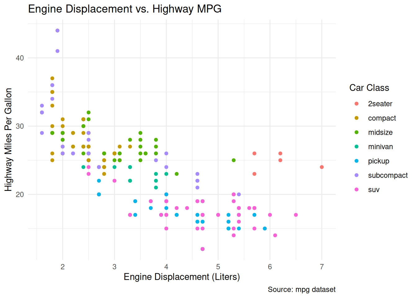
library(ggplot2)data(mpg) # Using the built-in mpg dataset# Scatter plot of engine displacement (displ) vs. highway mpg (hwy)# Colored by car classggplot(data = mpg, mapping =aes(x = displ, y = hwy, color = class)) +geom_point() +labs(title ="Engine Displacement vs. Highway MPG",x ="Engine Displacement (Liters)",y ="Highway Miles Per Gallon",color ="Car Class",caption ="Source: mpg dataset" ) +theme_minimal() # Apply a minimal theme
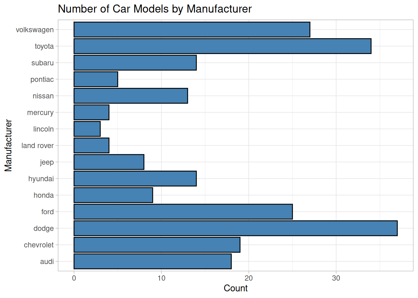
Example: Bar Plot Bar plots can represent counts or pre-summarized values.
# Bar plot of car counts by manufacturerggplot(data = mpg, mapping =aes(x = manufacturer)) +geom_bar(fill ="steelblue", color ="black") +# Counts are calculated by geom_barlabs(title ="Number of Car Models by Manufacturer", x ="Manufacturer", y ="Count") +theme_light() +coord_flip() # Flip coordinates to make manufacturer names readable
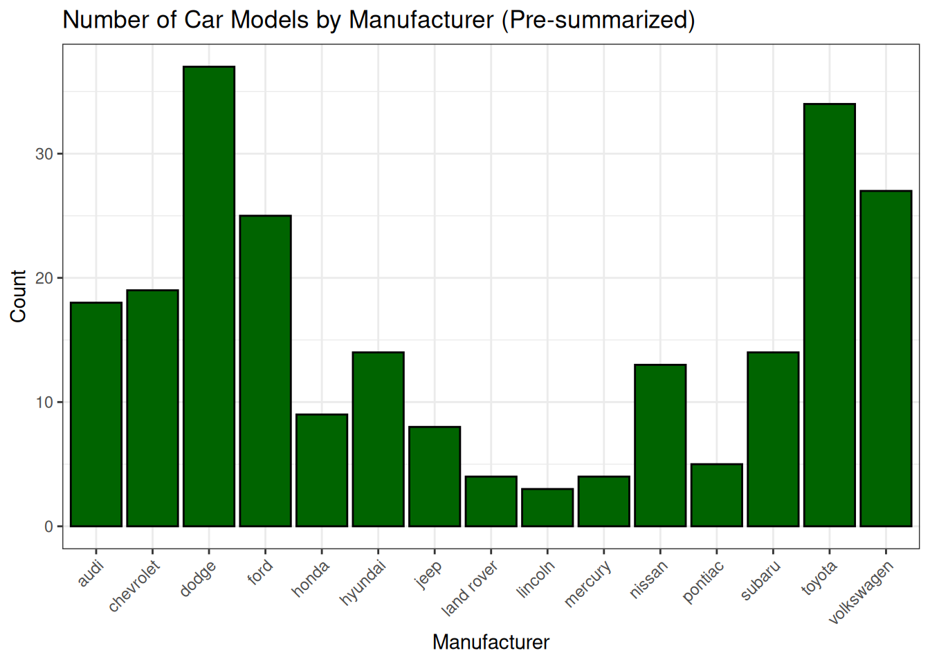
# If data is already summarized:manufacturer_summary <- mpg %>%count(manufacturer, name ="count")ggplot(data = manufacturer_summary, mapping =aes(x = manufacturer, y = count)) +geom_col(fill ="darkgreen", color ="black") +# Use geom_col for pre-summarized datalabs(title ="Number of Car Models by Manufacturer (Pre-summarized)", x ="Manufacturer", y ="Count") +theme_bw() +theme(axis.text.x =element_text(angle =45, hjust =1)) # Rotate x-axis labels
Exercise 6.1: Exploring Fuel Efficiency
Using the mpg dataset: 1. Create a scatter plot showing city miles per gallon (cty) vs. highway miles per gallon (hwy). 2. Color the points by drv (drive train: f=front, r=rear, 4=4wd). 3. Add a title and appropriate axis labels. 4. Experiment with geom_smooth(method = "lm") to add a linear regression line for each drv group.
Exercise 6.2: Distribution of Highway MPG
Create a histogram of highway miles per gallon (hwy).
Use facet_wrap(~ class) to create separate histograms for each car class.
Customize the bin width or number of bins for the histogram.
Add a vertical line representing the mean hwy for each class.
Lesson 7: Graphics II (Advanced {ggplot2})
Building on the essentials, we can further customize and enhance our {ggplot2} visualizations.
Scales
Scales control the mapping from data values to aesthetics. You can customize axes, colors, sizes, etc. * Position Scales (x and y axes): scale_x_continuous(), scale_y_continuous(), scale_x_discrete(), scale_y_discrete(), scale_x_log10(), scale_x_date(). * Control limits, breaks, labels. * Color and Fill Scales: scale_color_brewer(), scale_fill_brewer() (for discrete variables using ColorBrewer palettes), scale_color_gradient(), scale_fill_gradient() (for continuous variables), scale_color_manual(), scale_fill_manual() (for specifying colors manually). * Shape and Size Scales: scale_shape_manual(), scale_size_continuous().
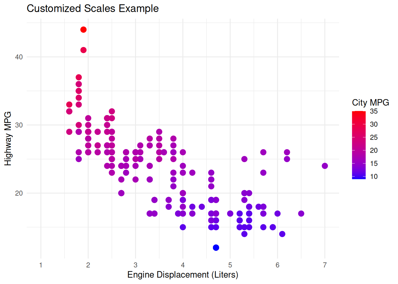
Example: Customizing Scales
ggplot(data = mpg, mapping =aes(x = displ, y = hwy, color = cty)) +geom_point(size =3) +scale_x_continuous(name ="Engine Displacement (Liters)",breaks =seq(1, 7, by =1),limits =c(1, 7) ) +scale_y_continuous(name ="Highway MPG",labels = scales::label_comma() # Use comma for thousands, etc. ) +scale_color_gradient(low ="blue", high ="red", name ="City MPG") +labs(title ="Customized Scales Example") +theme_minimal()
Themes
Themes control the non-data elements of the plot. * Built-in Themes: theme_gray() (default), theme_bw(), theme_minimal(), theme_classic(), theme_light(), theme_dark(), theme_void(). * Customizing Theme Elements: Use theme() to modify specific elements like plot.title, axis.text, axis.title, legend.position, panel.background, panel.grid.
Example: Custom Theme
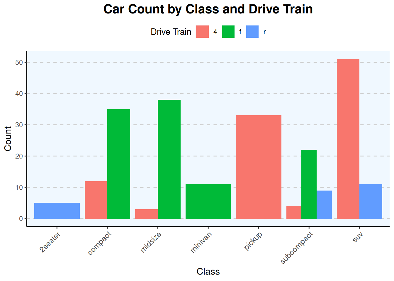
ggplot(data = mpg, mapping =aes(x = class, fill = drv)) +geom_bar(position ="dodge") +labs(title ="Car Count by Class and Drive Train", x ="Class", y ="Count", fill ="Drive Train") +theme_classic() +# Start with a classic themetheme(plot.title =element_text(hjust =0.5, size =16, face ="bold"),axis.text.x =element_text(angle =45, hjust =1, size =10),axis.title =element_text(size =12),legend.position ="top", # "bottom", "left", "right", "none", or c(x,y) coordinatespanel.grid.major.y =element_line(color ="grey80", linetype ="dashed"),panel.background =element_rect(fill ="aliceblue") )
Saving Plots: Use ggsave() to save plots to files (e.g., PNG, PDF, SVG). It infers the type from the extension.
Example: Annotations and Saving
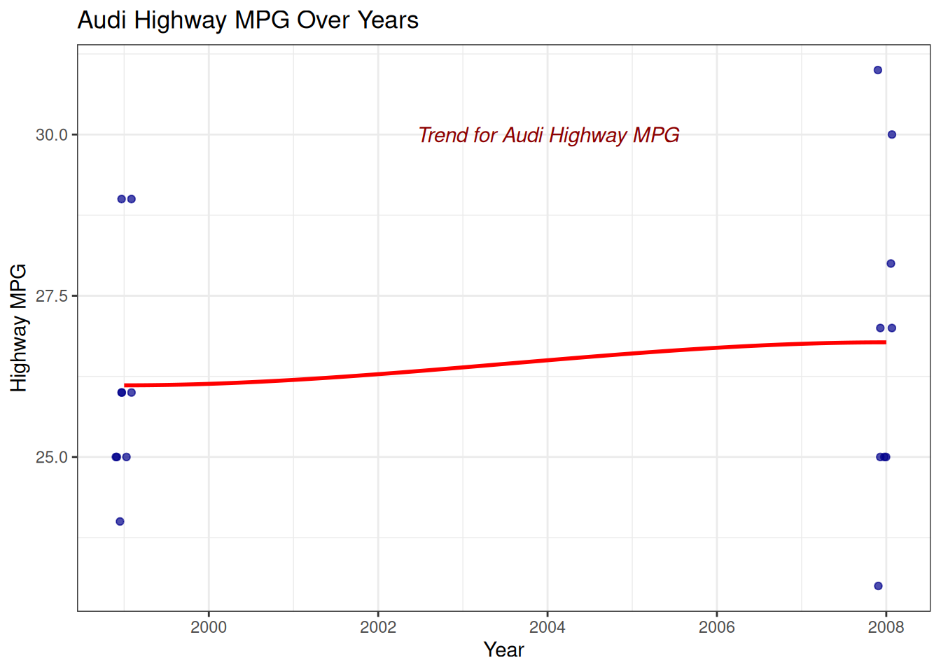
# This plot won't render in the QMD output directly if ggsave is used without printing the plot# For demonstration, we'll build it and then mention ggsave.p <-ggplot(data =filter(mpg, manufacturer =="audi"), aes(x = year, y = hwy)) +geom_jitter(width =0.1, height =0, alpha =0.7, color ="darkblue") +geom_smooth(method ="loess", color ="red", se =FALSE) +annotate("text", x =2004, y =30,label ="Trend for Audi Highway MPG",color ="darkred", fontface ="italic" ) +labs(title ="Audi Highway MPG Over Years", x ="Year", y ="Highway MPG") +theme_bw()print(p) # Display the plot
`geom_smooth()` using formula = 'y ~ x'
Warning in simpleLoess(y, x, w, span, degree = degree, parametric = parametric,
: pseudoinverse used at 1999
Using the mpg dataset: 1. Create a boxplot of hwy (highway MPG) grouped by class. 2. Fill the boxes based on drv (drive train). Use position = position_dodge(preserve = "single") if boxes overlap too much. 3. Customize the color palette for drv using scale_fill_brewer(palette = "Set2"). 4. Add a title: “Highway MPG Distribution by Class and Drive Train”. 5. Modify